DSP Speaker Recognition
Objective: Create a quasi-real time speaker recognition system using the Python programming language.
Speaker recognition (or voice recognition) is identifying the speech signal input as the person who spoke it. This is often confused with speech recognition which is the process of determining what vocabulary was used as opposed to who used it. Although very similar methods are used in each process, the algorithms that make sense of the extracted information are different.
There are two branches of speaker recognition: speaker identification and speaker verification. Identification determines exactly who is speaking and verification can simply state whether the speaker is a certain (predetermined) identity or not. Applications of these two types of speaker recognition range from personal and household assistants such as Amazon’s Alexa and Apple’s Siri to security such as allowing your voice to protect your bank account, etc. This project focuses on speaker identification.
|
Feature Extraction:
|
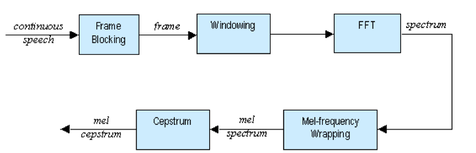
Block diagram for MFCC processor
|
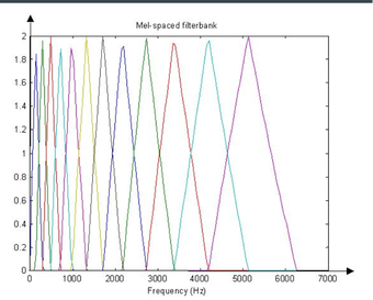 Mel filter bank
The feature extraction process is broken into 5 distinct parts in the figure above. Prior to entering the system, the input speech signal is sampled at 10kHz to get a discrete time signal which we are able to work with. The sampling rate was chosen to satisfy the Nyquist rate to avoid aliasing (highest speech frequency ≈3000Hz).
At this point we are ready to begin the first part of feature extraction which is frame blocking. In this step the input signal is blocked in the frames of N=256 samples. The overlap between the blocks is equal to N - M with M=100. The block length was chosen to be 25.6ms in length because it was found to be the optimal block size for getting usable frequency content. Too short of a duration results in unreliable spectral estimations and too large of a frame contains too much signal change to handle. After that the next step is to window the frames to minimize the discontinuities at the end points. This is done using a Hamming window of length N.
Now the process must move to the frequency domain. To do this we use the Discrete Fourier Transform (DFT) to convert each frame from time domain to the frequency domain. This transformation is implemented using the Fast Fourier Transform (FFT) function. Each block is 256 in length; the last one is zero padded if needed to reach that amount. The result of this step is a spectrum.
Next we need to identify which frequencies are present in each frame. The MEL filter bank allows us to get an idea of how much energy exists in the frequency regions. Spacing for it is linear below 1000 Hz and logarithmic above 1000 Hz. In total there are 20 filter banks, each one of them represents a mel spectrum coefficient K. This separation is done to model the human ear perception of hearing. It relates perceived frequency to the actual measured frequency. Humans are much better at discerning small changes in pitch at low frequencies than at high frequencies. The picture above shows a depiction of what this filter bank looks like. Each filter can be viewed as a histogram bin in the frequency domain.
The final step is to convert the log mel spectrum back to the time domain (mel-frequency cepstrum). This is done by calculating the discrete cosine transform. The reason for using this is, the Mel Spectrum Coefficients are all real numbers. The result of transforming the Mel Frequency Cepstral coefficients (MFCC) back to the time domain is the Mel Power Spectrum. The Mel Power Spectrum is a short-term power spectrum expressed on the mel-frequency scale. The Mel Power Spectrum is called an acoustic vector and will be the input to our feature matching system.
Feature Matching:
In the feature extraction section, we train the system with information about different speakers. Now it is time to identify who is speaking in the feature matching section.
A few definitions before moving forward.
Training set: patterns provided to derive a classification algorithm.
Test set: patterns used to test classification algorithm.
Vector Quantization (VQ): is the process of mapping vectors from a large vector space to a finite number of regions in that space.
Cluster: name for each region in space.
Codeword: the center of a cluster.
Codebook: a collection of all codewords.
Q-distortion: the distance from a vector to the closest code word of codebook.
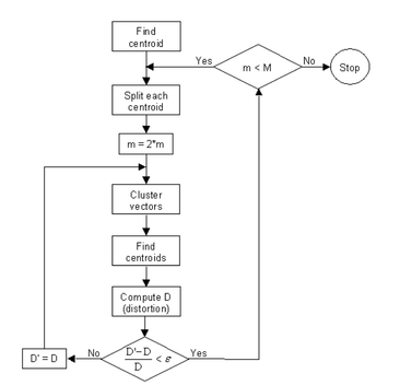
Flow diagram of LBG algorithm
|
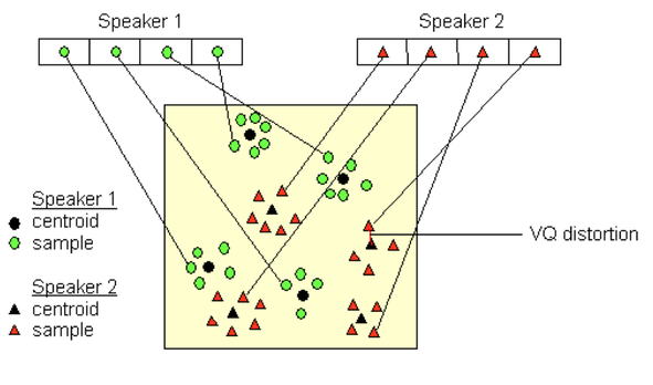
Vector quantization codebook information
|
To cluster the training vectors the Linde Buzo Grey (LBG) algorithm is used for clustering a set of L training vectors into a set of M codebook vectors. Above shows the recursive procedure. The first step is to design a 1-vector codebook to be the centroid of the entire set of training vectors. Next the codebook is doubled in size by splitting each codebook. After that, the nearest neighbor search method is applied to each training vector to find the codeword in the current codebook that is closest. Then the vector is aligned to that corresponding cell. Step four is to update the codeword in each cell using the centroid of the training vectors assigned to that cell. Next you enter the first iteration decision until the average distance falls below a preset threshold ε. When you fall out of that, you enter iteration 2 which runs until a codebook of size M is designed.
The figure above is a conceptual illustration representing the recognition process. It represents two speakers, with circles corresponding to speaker 1 and triangles corresponding to speaker 2. Using the LBG algorithm, a speaker-specific vector quantized codebook is generated for each known speaker by clustering their training acoustic vectors. The resulting codewords are shown in the figure above as black circles and individual speakers are shown as triangles. The distance from a vector to the closest codeword of a codebook is known as VQ-distortion. To identify a speaker, the unknown voice is vector quantized using each trained codebook, the total VQ distortion is computed. The speaker corresponding to the VQ codebook with the smallest total distortion is identified as the speaker of the input signal.
The figure above is a conceptual illustration representing the recognition process. It represents two speakers, with circles corresponding to speaker 1 and triangles corresponding to speaker 2. Using the LBG algorithm, a speaker-specific vector quantized codebook is generated for each known speaker by clustering their training acoustic vectors. The resulting codewords are shown in the figure above as black circles and individual speakers are shown as triangles. The distance from a vector to the closest codeword of a codebook is known as VQ-distortion. To identify a speaker, the unknown voice is vector quantized using each trained codebook, the total VQ distortion is computed. The speaker corresponding to the VQ codebook with the smallest total distortion is identified as the speaker of the input signal.
MATLAB:
Our first implementation to test our voice recognition system was done using MATLAB. The process was split into a training and testing phase. Within the training phase we input a set of .wav files of different speakers to use as our training set. Once those were processed, a reference codebook was generated for us to compare with in the testing phase.
For the testing phase, we input our reference codebook into the system along with new .wav files of speakers to identify. The output of the system is the reference signal that matches each new .wav file identifying the speaker.
Python:
To achieve our desired goal of having a real time voice recognition system, we decided to use the programing language Python instead of MATLAB. Python scripts do not require the large overhead that MATLAB GUI needs. Python also is easy to integrate with existing hardware on the computer. We will be needing it to interface with the microphone on our laptops to record user audio. Finally it can be compiled into a single executable which allows us freedom from a backend application. All of these qualities make Python desirable for our real time voice recognition application.
To transfer the project to python, we found two useful libraries―numpy and scipy―that have many of the array manipulations and mathematical commands similar to MATLAB. For example: in MATLAB, one can easily allocate a certain number of elements to a vector, but that is not easily doable with standard python. Numpy has the command numpy.zeros() which has essentially the same functionality as the MATLAB command.
One challenge of developing a real-time system with input speech signals and manipulation, is collecting data while analyzing for speaker recognition. We addressed this issue by choosing to use only small segments of time (about 0.2 seconds) and quickly computing the acoustic vector, followed by the distance to the codewords in the codebook.
There are some drawbacks to this method. One being, speech in between computations that is not recorded. In addition to this, there will be far less variation in the acoustic vectors because of the short length of the segment of time. If the 0.2 seconds of speech is uncharacteristic of the individual’s overall voice, the system will likely be unable to identify them correctly.
Results:
Using the sample data provided in the lab, we tested our MATLAB system.
This training directory contains 8 different speakers saying the word “zero”. Each file is used as input to our training system by running the command.
>> code=train('traindir\',8);
traindir\s1.wav
traindir\s2.wav
traindir\s3.wav
traindir\s4.wav
traindir\s5.wav
traindir\s6.wav
traindir\s7.wav
traindir\s8.wav
The function parameters are the directory where the files are found and how many files that directory contains.
After the training is complete, the testing phase begins by inputting the generated codebook “code” as a reference to the new speaking data. The testing directory contains those 8 speakers saying the word “zero” at a different time.
>> test('testdir\',8,code);
Speaker 1 matches with speaker 1
Speaker 2 matches with speaker 2
Speaker 3 matches with speaker 7
Speaker 4 matches with speaker 4
Speaker 5 matches with speaker 5
Speaker 6 matches with speaker 6
Speaker 7 matches with speaker 7
Speaker 8 matches with speaker 8
The function parameters are the directory where the files are found, how many files that directory contains and the reference codebook. The results are printed below the command and show which speaker matched with whom. The first speaker is the test speaker and the matched speaker is the one trained into the system. It can be seen that it correctly matched ⅞ times. The reason for this discrepancy is that the system matches the closest and since the test signals were taken at a different time, many variables come into play. Voices change over time, sickness affects the way we sound, or the environment in which it was recorded changed. These possibilities and more could be the reason for the mistake with speaker 3 matching with speaker 7.
Now we decided to test the system with our own voices.
>> code=train('testdir2\',2);
testdir2\s1.wav
testdir2\s2.wav
In this example, Alex is the odd speaker and Tim is the even speaker. We say a few words that incorporate a range of the 44 sounds in the English language. We decided on words that had 5 of the short vowel sounds. The short-a- in “after”, short -e- in “lend”, short -i- in “in”, short -o- in “hop”, and short -u- in “cup”. The system was then tested with a new word that was not trained. The word we chose was “pen”, this has the short -e- sound and we hoped that it detected the correct speaker as that sound should be trained in with the word “lend”.
System is tested with the word “pen”
>> test('testdir2\',2,code);
Speaker 1 matches with speaker 1
Speaker 2 matches with speaker 2
This time the system matched 100% by pairing the correct speaker with the correct reference.
Next the system was tested again with the testing directory of us saying “zero” in a few different tones to see if it would still match our voice.
>> test('testdir1\',4,code);
Speaker 1 matches with speaker 1
Speaker 2 matches with speaker 2
Speaker 3 matches with speaker 1
Speaker 4 matches with speaker 2
Again Alex is the odd speaker and Tim is the even speaker. It can be seen that once again the system matched with 100%.
It was found that for a low set of speakers the system worked very well by identifying who was closest to the reference signals.
|
We were able to build a system in Python that would record audio and automatically trim the file to regions of content. It would then write to a .wav file that would be used to do the testing on. The code for each of the MATLAB functions was written in attempts to convert it over to Python. It was difficult to deal with matrices in Python and tedious to get the same functionality out of the program. We did not have enough time to complete the debugging process in a few of the programs so we were unable to get a fully working program. To the right, shows some screenshots of the functionality of the program.
In the example to the right (results 1), the black text is user input and the blue is the program prompts. |
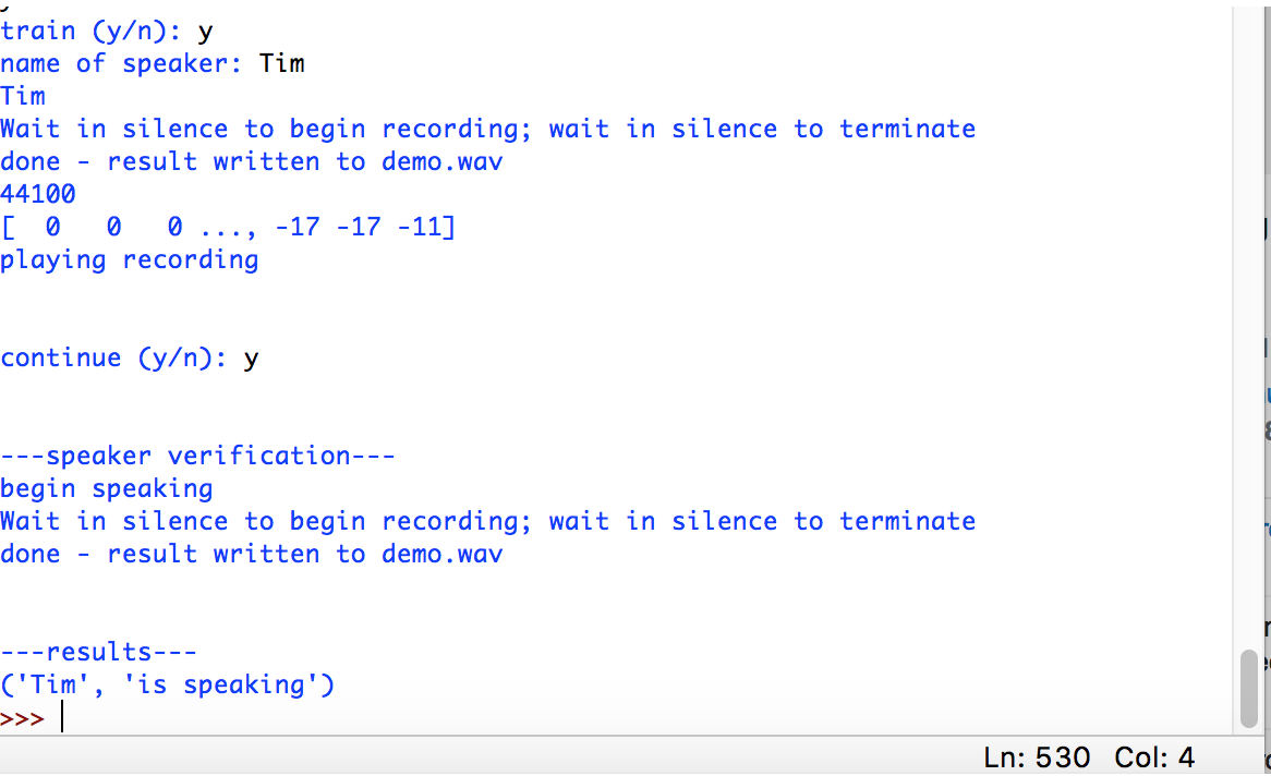
results 1
|
|
The system prompts for training or testing phase and asks for a name, then saves recording. After the name is recorded it can be tested to see if it can figure out who is speaking.
The image to the right (results 2), shows Tim recording the work “hello” and Alex recording the word “hello”. Afterwords, the user enters the verification process and Alex begins speaking “hello”, the system responds by stating that “Alex” is the one speaking. In the future when we have more time we would like to make a better user interface for the program and have the option to load in a training file instead of re-recording each time. This will require additional time debugging to get the system working like it did in MATLAB. |
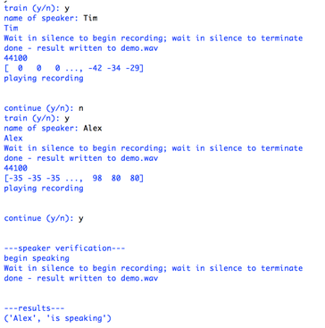
results 2
|
Conclusion:
Speaker recognition was a great project to demonstrate a few of the concepts we learned throughout DSP. The blocking, windowing, overlapping, and DFT of a signal is more better understood than if we had not taken the class. The Mel-Frequency Cepstrum is also a useful tool that we now have because it can characterize a speech signal. In addition to these concepts, we also have some experience using Python―a language that is generally a more desirable programming language than MATLAB. If we were to do something differently, we might take a different approach than the Mel Frequency Spectrum. There are several other ways to implement a speaker recognition system (such as deep neural networks) that are even more accurate.
Implementation highlighted below in slides
| 424_project.pdf |
